Hydroelasticity

Recently I visited Harbin, China to attend a PhD summer school on Ocean Engineering which was organized by the University of Dundee and Harbin Engineering University. The scientific topic of the Summer School was Hydroelasticity of Fixed and Floating Bodies. The summer school contained lectures on hydroelasticity and soon after we were assigned a group project at the end of the summer school.

The entire analysis was performed using ANSYS and Hydran-XR. However, in a series of upcoming blog posts, I aim to describe the entire procedure in a detailed manner explaining the governing equations and the finite element method to solve the problem. Let’s set sailing (Pun intended)…

The problem is to determine the hydroelastic response of a boat whose hull shape is given by the surface,

\[\begin{equation} y = \frac{1}{2}B\left(1-\frac{4x^2}{L^2}\right)\left(1-\frac{y^2}{d^2}\right) \end{equation}\]

with \(-L/2<x<L/2\) and \(-d<z<d\). To be helpful, I give you a quick MATLAB script to plot the shape of the hull.

clear
L = 100; B = 10; d = 2.25;

x = linspace(-L/2,L/2,20);
z = linspace(-d,0,20);
[X,Z] = meshgrid(x,z);

Y = 1/2*B*(1-4*X.^2/L^2).*(1-Z.^2/d^2); % The hull

surf(X,Y,Z,'edgecolor','none');
axis equal
hold on
surf(X,-Y,Z,'edgecolor','none');

Discretization of the Domain

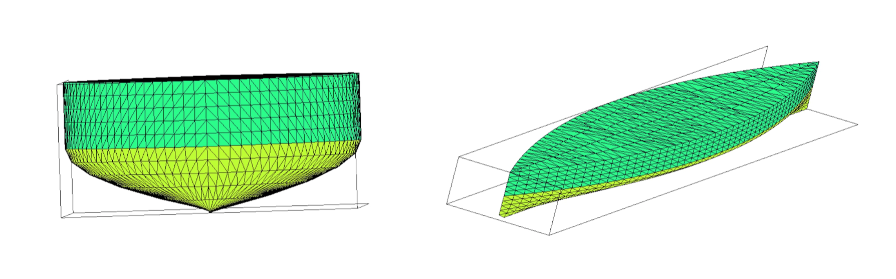
To use the finite element method, we need to obtain the finite element mesh of the computational domain. The mesh generator of FreeFem++ is quite handy to obtain tetrahedral meshes. After placing a deck over the hull (which has a uniform height), we generate the mesh using Freefem++. I have been playing around with a few visualization tools like Gmsh and ffmedit and found out that Gmsh, although extremely versatile has a steep learning curve, whereas ffmedit is quick and simple. Below, I show the oblique and front view of the assembled structure.

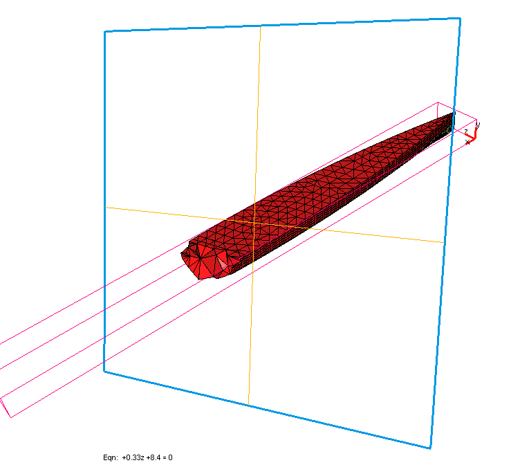
Now to view the tetrahedrons in the mesh, I use ffmedit to clip the mesh along a plane. Then, ffmedit displays the tetrahedrons along the cross section made by the plane. The plane of view can be fixed and the body can be rotated to view the tetrahedrons which can be done with ease.

Now, once the appropriate finite element mesh is obtained, we proceed to the first part in the hydroelastic analysis - which is to obtain the in-vacuo/dry modes.

Dry Modes

In linear hydroelasticity, often a reduced basis is preferred more than the finite element basis to obtain the solution due to simplicity in obtaining the linear system. These reduced basis comes in the form of dry modes/in-vacuo modes which are obtained as follows.

The object of interest \(\Omega\) is taken out of the water and put in vacuum. The body does not experience any hydrostatic force and thus the body forces and tractions on the surface is zero. The vibration of the system is governed by the boundary value problem

\[\begin{eqnarray} -\nabla \cdot \sigma(u) &=& \beta^2 u \quad \text{in } \Omega\\ \sigma\cdot\mathbf{n} &=& 0 \quad \text{on } \partial\Omega \end{eqnarray}\]

where \(\sigma\) is the Cauchy stress tensor and \(\mathbf{u}\) is the displacement field. Let us call by \(\mathcal{T}_h\), the finite element mesh we generated above. So we define a finite element space

\[V_h = \left\{ v \in [H^1_0(\Omega)]^2 \; : \; v \in \mathbb{P}_1(K),\, \forall K\in\mathcal{T}_h \right\}.\]

which simply means that we use linear approximations for the solution. The dry modes are the solution to the above boundary value problem whose weak formulation is to find \(u_h \in V_h\) such that

\[\int_{\Omega} \sigma(u_h) : \epsilon(v_h) \,dx = \beta^2\int_{\Omega}u_h\cdot v_h\,dx, \qquad \forall v_h \in V_h\]

or in matrix form

\[[\mathbf{K}-\beta^2\mathbf{M}]\{u_h\} = 0\]

The reduced basis can be obtained as the solution to this eigenvalue problem which in turn are obtained using FEM. The eigenvalues \(\beta^2\) are the natural frequency of the system and the corresponding eigenfunctions are the mode shape associated with the natural frequency. The problem can be quickly solved using FreeFem++.

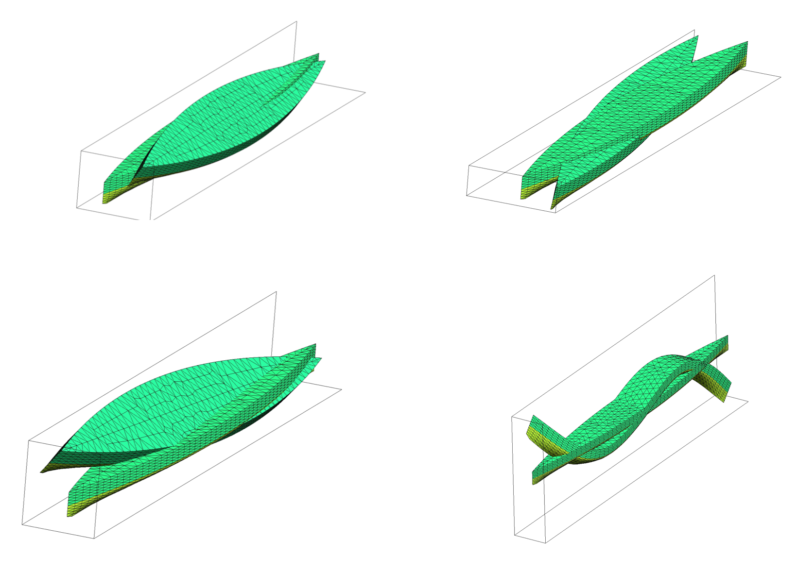
Table below shows the first ten eigenvalues obtained. Since we study the free-vibrations of the body, the first 6 vibration modes are rigid body modes (meaning you won’t observe any elastic deformation. See figure below) and the eigenvalues are equal to 0 (machine precision). In ocean engineering they are usually named heave, roll, pitch, yaw, sway, surge (Not in any particular order)

Mode	Eigenvalue
(1)	7.62406e-17
(2)	-2.44254e-16
(3)	-1.03438e-15
(4)	-1.3254e-15
(5)	1.3761e-15
(6)	2.07506e-15
(7)	0.000670548
(8)	0.00156645
(9)	0.00315441
(10)	0.00673546

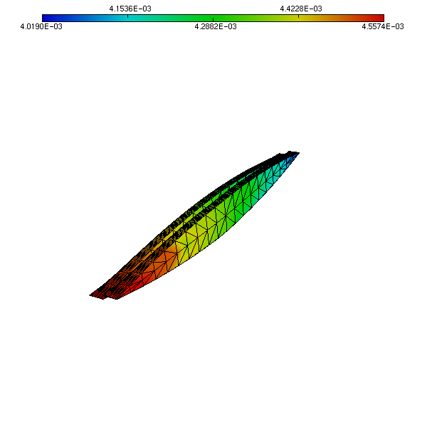
Figure below shows the first three rigid body modes and the 9th elastic vibration mode for the object.

This can be used as a reduced basis to solve the response of a boat sailing in ocean. The following Figure shows the \(z-\) derivative of the velocity potential which indirectly shows the free-surface elevation \(\eta(x,y)\)

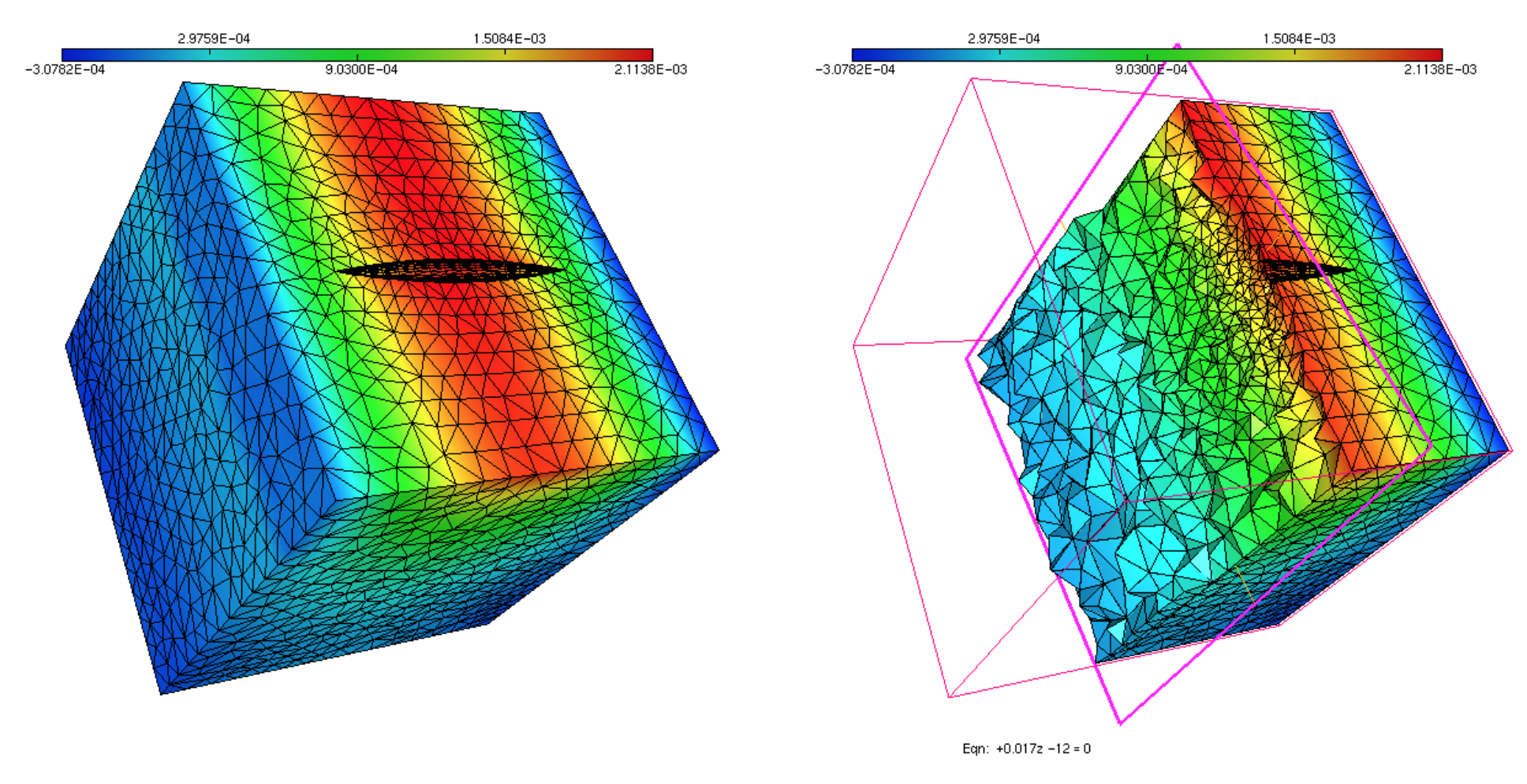
given by the kinematic relation,

\[\begin{equation} \partial_z\phi = -i\omega\,\eta, \end{equation}\]

for a given incident frequency. The following Figure shows the vertical displacement of the boat for the same incident frequency.

Overall, the summer school has been a wonderful experience, an gave me an opportunity to meet a lot of fellow PhD students working in Ocean Engineering and allied topics.