
Postdoc at Umeå University, Sweden
Virtual elements, biorthogonal projections and the peculiarity of second order VEM
When I began writing this post on 26th November, I was on a train from Wollongong to Newcastle. Being a long ride back home, I decided to work on this blog post about VEM. But I ended up finishing and pushing this post on 5th December.
This one is going to be a bit long and slightly technical, but the results are quite interesting and the questions that arise at the end of this post gives us new insight into the construction of the virtual element method. I will be covering four major topics here which will leave us with three mind blowing moments.
- Overview of the older mixed method.
- Mixed Method based on bi-orthogonal systems.
- Why is the stability term required here but not for gradient recovery?
- What is so interesting about second order/quadratic VEM?
Mixed method for fourth order problem
In the last post, I proposed a modified gradient recovery approach using a stability term. At the end of the post, I mentioned about how this stability term is important in some cases. When I was talking about gradient recovery techniques to my one of my supervisors, he suggested me to look at another application of bi-orthogonality for constructing mixed methods using the Ciarlet-Raviart formulation.
Let us consider the fourth-order biharmonic equation
\[\begin{equation} \Delta^2 u = f, \quad \text{in}\quad \Omega \end{equation}\]with \(\Delta(\cdot)\) denoting the standard Laplacian operator. The idea in a Ciarlet-Raviart mixed formulation is to construct a mixed method by considering an auxiliary variable \(v = -\Delta u\) and thus transform the problem into a system of two second order problems
\[\begin{eqnarray*} -\Delta v &=& f,\\ -\Delta u &=& v. \end{eqnarray*}\]As for the boundary condition let us assume that
\[u = \frac{\partial u}{\partial n} = 0 \quad \text{on}\;\; \partial\Omega.\]In usual mixed formulations, we deal with weak formulations that are constructed using the above PDEs as to find \((u,v) \in H^1_0(\Omega) \times H^1(\Omega)\) such that
\[\begin{eqnarray*} (\nabla v, \nabla \varphi) &=& (f,\varphi),\\ (\nabla u, \nabla \chi) &=& (v,\chi), \end{eqnarray*}\]for all \((\varphi,\chi) \in H^1_0(\Omega)\times H^1_0(\Omega)\). Note that the derivative boundary condition occur naturally in the formulation. Let \(S_h\) denote the standard linear virtual element space and \(S_h^0\) denote the same virtual element space with zero value on the boundary. Due to the virtual element discretization, we arrive at the following discrete equivalent.
Find \((u_h,v_h) \in S_h^0\times S_h\) such that
\[\begin{eqnarray} a_h(v_h,\varphi) &=& f_h(\varphi),\\ a_h(u_h,\chi) &=& m_h(v_h,\chi). \end{eqnarray}\]\((\varphi,\chi) \in S_h \times S_h\). Then we have the system of equations
\[\begin{bmatrix} 0 &K\\ -K &M \end{bmatrix} \begin{Bmatrix} u\\ v \end{Bmatrix} = \begin{Bmatrix} f\\ 0 \end{Bmatrix}\]which after applying the Dirichlet boundary conditions for \(u\), can be solved to obtain the solution. Although inverting the sparse left hand side matrix is relatively simpler than implementing a \(C^1\) finite element method, we could do better if we implement bi-orthogonal systems.
Mixed method using bi-orthogonal systems
The original paper [1] describes the procedure based on energy functionals and saddle point theory. I will present here, an easier and intuitive approach. We start by splitting the fourth order problem into two second order problems as
\[\begin{eqnarray*} \Delta u &=& \phi,\\ \Delta \phi &=& f. \end{eqnarray*}\]We further split the second equation into two equations by setting \(\phi = -p\) and writing
\[\begin{eqnarray*} -\Delta p = f. \end{eqnarray*}\]Define the spaces
\[\begin{eqnarray*} V &=& H^1_0(\Omega) \times L^2(\Omega),\\ Q &=& H^1(\Omega) \end{eqnarray*}\]and the virtual element subspaces \(V_h \subset V\) and \(Q_h \subset Q\), where
\[V_h = S_h^0 \times M_h, \quad Q_h = S_h.\]The discrete virtual element setting reads: Find \(((u_h,\phi_h),p_h) \in V_h \times Q_h\) such that
\[\begin{eqnarray*} a_h(p_h,v) &=& f_h(v),\\ a_h(u_h,q) &=& m_h(\phi_h,q),\\ -m_h(\phi_h,\psi) &=& m_h(p_h,\psi), \end{eqnarray*}\]where \(((v,\psi),q) \in V_h \times Q_h\). Written in matrix form, we obtain the system of equations
\[\begin{eqnarray*} \begin{bmatrix} K & D & 0\\ 0 & -M & D^T\\ 0 & 0 & K^T \end{bmatrix} \begin{Bmatrix} u\\ \phi\\ p \end{Bmatrix} = \begin{Bmatrix} 0\\ 0\\ f \end{Bmatrix}. \end{eqnarray*}\]Further, we can statically condense out the variable \(u\) as
\[\begin{eqnarray*} \left(K^T (D^T)^{-1} \,M\,D^{-1} K\right)\,u &=& f,\\ \end{eqnarray*}\]and after solving for \(u\), we can find
\[\begin{eqnarray*} \phi &=& -\left(D^{-1}\,K\right)\,u,\\ p &=& \left( (D^T)^{-1} \,M\, D^{-1} K \right)\,u. \end{eqnarray*}\]Now, what is this space \(M_h\)?? Choosing \(M_h\) as the space of functions bi-orthogonal to the virtual element space \(S_h\), the matrix \(D\) becomes diagonal! And inverting a diagonal matrix is the easiest and the sweetest thing to do computationally (Mind blown)… To put it formally, define
\[M_h = \text{span}\{\mu_1,\mu_2,\cdots,\mu_N\},\]with
\[\int_K \varphi_i\,\mu_j = c_j\delta_{ij},\]for all the virtual elements \(K\). The coefficients \(c_j\) can be chosen proportional to the area of the element and is given by the mass-lumping. The interesting part is yet to come…
Stability term
On closer inspection of the weak form, we find that the discrete inner product
\[m_h(\mu_i,\mu_j) = \sum_K m_h^K(\mu_i,\mu_j)\]needs to satisfy good stability properties in the virtual element setting. To achieve this, the local bilinear form needs to satisfy the following lower and upper bound
\[C_1\|v_h\|_{0,K}^2 \le m_h^K(v_h,v_h) \le C_2 \|v_h\|_{0,K}^2\]The local \(L^2\) inner product is defined as
\[m_h^K(\mu_i,\mu_j) = \int_K \Pi^0_K\mu_i\, \Pi^0_K\mu_j + T_K\]The \(L^2-\) projection \(\Pi^0_K\mu_j\) can be fully computed using the bi-orthogonal relation (It is a really cool exercise to work it out). The stability term \(T_K\) needs to be only approximated and can be chosen to be equal to the one described in the previous post.
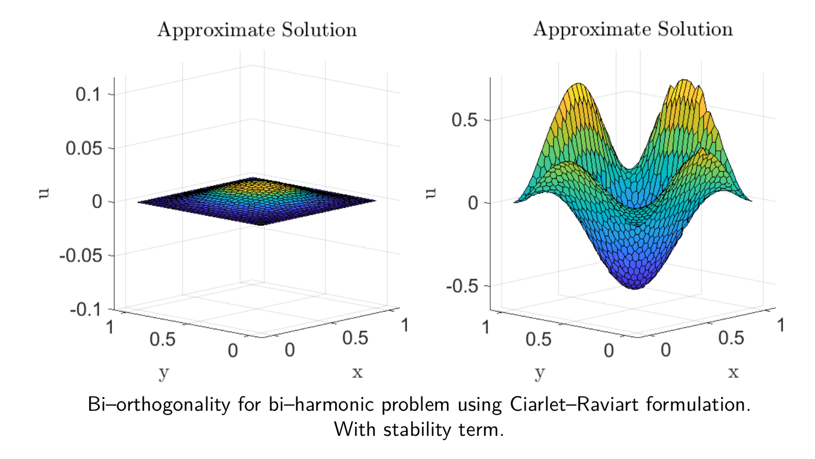
Visually, when the stability term is ignored, we have an unstable solution to the stream function \(p\),
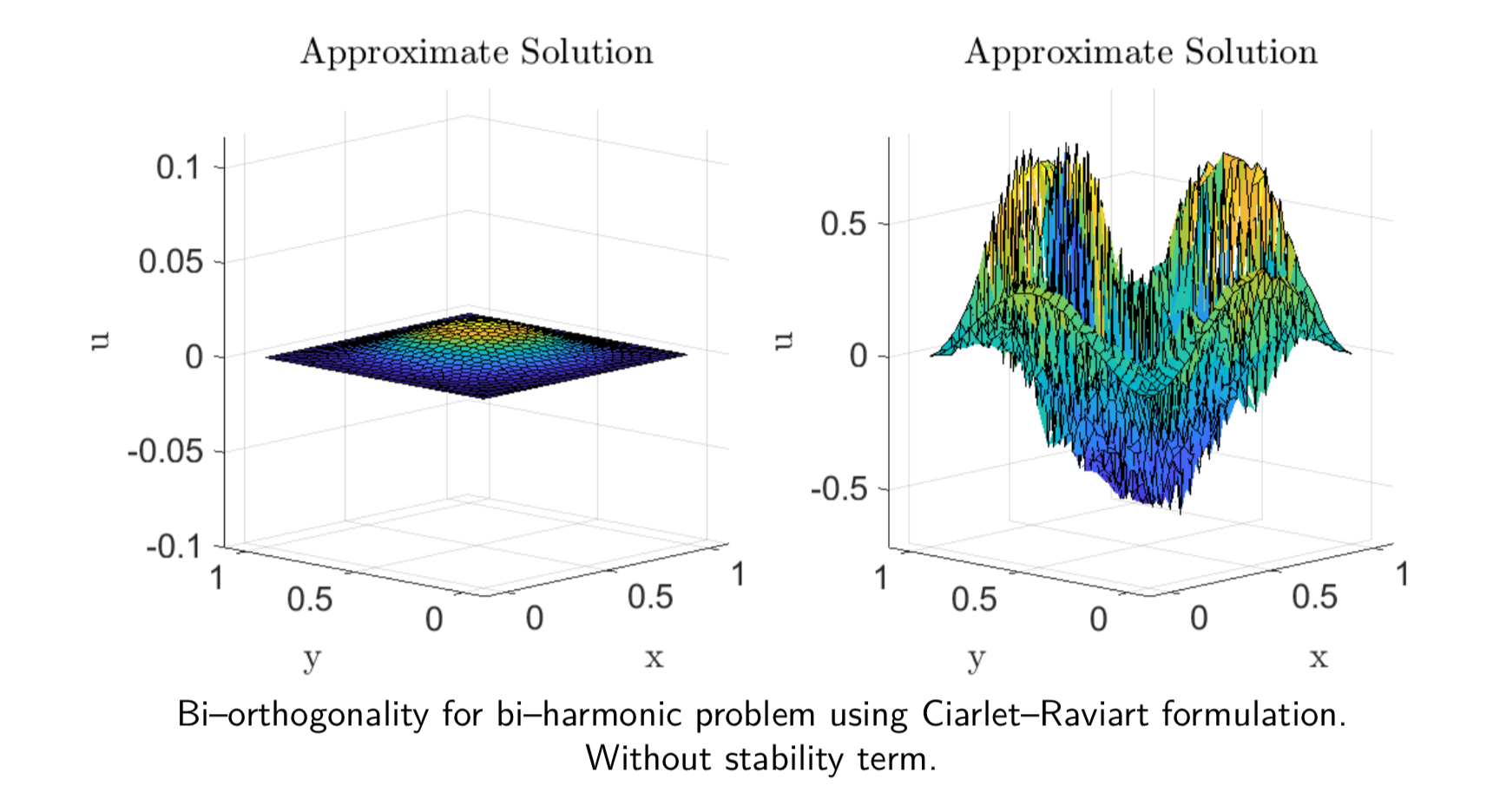
However, when we add the stability term we obtain a much cleaner solution. Since we do not require the lower bound in the gradient recovery case, we can ignore the stability term there (Mind blown … Again).
Peculiarity of the second order VEM
What is so peculiar about the quadratic virtual elements now? Before answering this question, let us go back to the definition of the bi-orthogonal bases. Define
\[M_h = \text{span}\{\mu_1,\mu_2,\cdots,\mu_N\},\]with
\[\int_K \varphi_i\,\mu_j = c_j\delta_{ij},\]for all the virtual elements \(K\). The coefficients \(c_j\) can be chosen proportional to the area of the element and is given by the mass-lumping.
Turns out second order VEM does not get along very well with mass-lumping. Why? Applying the mass lumping technique the elements of the diagonal matrix are given as
\[\begin{eqnarray*} c_j &=& \sum_{i=1}^{N} \int_K \varphi_i \,\varphi_j\\ &=& \int_K \left(\sum_{i=1}^{N} \varphi_i\right) \,\varphi_j\\ &=& \int_K \varphi_j \end{eqnarray*}\]However, the integral of the bases function is taken as the first moment degree of freedom in the quadratic virtual element setting. This means the local lumped mass matrix, for example, for a any polygon takes the form
\[\begin{bmatrix} 0 & \cdots & 0\\ \vdots & \ddots & \vdots \\ 0 & \cdots & |K| \\ \end{bmatrix}\]which after assembly cannot be inverted (Mind.. blown.. Again..)
What now? No Idea. But the remedy will be a subject of a future blog post. So stay tuned ;)
References
[1] Lamichhane, Bishnu P. “A mixed finite element method for the biharmonic problem using biorthogonal or quasi-biorthogonal systems.” Journal of Scientific Computing 46.3 (2011): 379-396.
[2] Kalyanaraman, B., Lamichhane, B., & Meylan, M. (2018). A gradient recovery method based on an oblique projection for the virtual element method. ANZIAM Journal, 60, 201-214.
tags: wip - vem - biorthogonal - projection - VEM © 2019- Balaje Kalyanaraman. Hosted on Github pages. Based on the Minimal Theme by orderedlist