
Postdoc at Umeå University, Sweden
Mixed DG methods for Biharmonic Equation
Let us take the biharmonic problem on \(\Omega\) along with the clamped conditions on the boundary \(\partial\Omega\).
\[\begin{align} \Delta^2 u = f \quad &\text{in }\Omega\\ u = \nabla u\cdot \mathbf{n} = 0 \quad &\text{on } \partial\Omega \end{align}\]We now split the biharmonic equation into two equations by introducing an auxiliary variable \(v = \Delta u\). We then have a system of equations
\[\begin{align} \begin{cases} \Delta u &= v \\ \Delta v &= f \end{cases}\quad &\text{in }\Omega\\ u = \nabla u\cdot \mathbf{n} = 0 \quad &\text{on } \partial\Omega \end{align}\]The system is a little tricky to solve since, we do not have a boundary condition on \(v\). It is possible to come up with a discontinuous Galerkin weak formulation, as discussed by Gudi, T., Nataraj, N. & Pani, A.K in their article. I will briefly discuss the construction of their scheme and how a simple modification leads to an increased rate of convergence.
Mixed DG Method
Let us divide the domain \(\Omega\) into shape regular finite elements (consider triangles). Let
\[\mathcal{T}_h = \cup_{i=1}^{N_T} K_i\]denote the triangulation of the domain, with \(K_i\) denoting the \(i\)-th triangle on the domain. Let us denote by \(\Gamma_\text{I}\) the set of all interior edges, and \(\Gamma_\text{D}\) the set of all boundary edges. Let \(\Gamma = \Gamma_\text{I} \cup \Gamma_\text{D}\). For each edge \(e_k = \partial K_i \cap \partial K_j\), associate a unit normal \(n_k\). Note that the triangulation can contain hanging nodes along each side of the elements.
Since we are dealing with discontinuous functions, we require functions from the “broken” Sobolev space,
\[H^s(\Omega, \mathcal{T}_h) = \left\{ v \in L^2(\Omega) \,:\, v |_{K_i} \in H^s(K_i) \; \forall K_i \in \mathcal{T}_h\right\}\]Let \(V = H^2(\Omega, \mathcal{T}_h)\). The jump and average of a function \(v\) across the edge \(e_k = \partial K_i \cap \partial K_j\) are defined as
\[\begin{align} [v] &= v|_{K_i} - v|_{K_j}\\ \{v\} &= \frac{v|_{K_i} + v|_{K_j}}{2} \end{align}\]There are other intricate assumptions on the triangulation which can be found in the article. But we have all the necessary ingredients to define the mixed DG method.
-
Let us take the first equation,
\[\Delta u = v\]multiply by a function \(w \in V\) and integrate over the domain
\[\int_\Omega (- \Delta u + v)w\,dx = 0\]As usual proceeding with integration by parts, we obtain
\[\begin{align} \sum_{K\in \mathcal{T}_h}\int_K \nabla u\cdot \nabla w\,dx - \sum_{e_k \in \Gamma_\text{I}} \int_{e_k} \left\{\frac{\partial u}{\partial n_k}\right\}[w]\,ds + \int_\Omega u\,v\,dx = 0 \end{align}\]Here we have used the fact that \(\nabla u \cdot \mathbf{n} = 0\) on \(\Gamma_\text{D}\). For a sufficiently smooth function \([u] = 0\) on \(\Gamma_{\text{I}}\) and also since \(u = 0\) on the boundary, adding the term
$$ \begin{align} \sum_{K\in \mathcal{T}_h}\int_K \nabla u\cdot \nabla w\,dx - \sum_{e_k \in \Gamma_\text{I}} \int_{e_k} \left\{\frac{\partial u}{\partial n_k}\right\}[w]\,ds - \color{red}{\sum_{e_k \in \Gamma} \int_{e_k} \left\{\frac{\partial w}{\partial n_k}\right\}[u]\,ds} + \int_\Omega u\,v\,dx = 0 \end{align} $$does not affect the equation. If \(u = g_1(x) \ne 0\) on the boundary, then the term containing the weakly imposed DBC will appear on the RHS.
-
Similarly with the second equation,
\[\Delta v = f\]multiply a function \(q \in V\) and integrate over the domain
\[\int_\Omega (-\Delta v + f)q \,dx = 0\]Applying integration by parts,
\[\begin{align} \sum_{K\in \mathcal{T}_h} \int_K \nabla v\cdot \nabla q\,dx - \sum_{e_k \in \Gamma} \int_{e_k} \left\{\frac{\partial v}{\partial n_k}\right\}[q]\,ds = -\int_\Omega fq\,dx \end{align}\]For a sufficiently smooth function \(v\), we have \([v]=0\) on \(\Gamma_\text{I}\). We can add the term shown in red. Also like before, for a sufficiently smooth function \([u] = 0\) on \(\Gamma_{\text{I}}\). Since \(u=0\) on the boundary also, we can add the term shown in blue. The latter imposes the DBC weakly.
$$ \begin{align} \small \sum_{K\in \mathcal{T}_h} \int_K \nabla v\cdot \nabla q\,dx - \sum_{e_k \in \Gamma} \int_{e_k} \left\{\frac{\partial v}{\partial n_k}\right\}[q]\,ds - \color{red}{\sum_{e_k \in \Gamma_\text{I}} \int_{e_k} \left\{\frac{\partial q}{\partial n_k}\right\}[v]\,ds} - \color{blue}{\sum_{e_k \in \Gamma} \int_{e_k} \alpha \,[u][q]\,ds} = -\int_\Omega fq\,dx \end{align} $$
To clean things up a bit, let us define the bilinear forms
\[\begin{align} B(w,q) &= \sum_{K\in \mathcal{T}_h} \int_K \nabla w\cdot \nabla q\,dx - \sum_{e_k \in \Gamma} \int_{e_k} \left\{\frac{\partial w}{\partial n_k}\right\}[q]\,ds - \sum_{e_k \in \Gamma_\text{I}} \int_{e_k} \left\{\frac{\partial q}{\partial n_k}\right\}[w]\,ds\\ J(w,q) &= \sum_{e_k \in \Gamma} \int_{e_k} \alpha \,[w][q]\,ds \end{align}\]A mixed weak formulation of the biharmonic problem is to find \((u,v) \in V\times V\)
\[\begin{align} B(w, u) + (u,v) &= 0,\\ B(v, q) - J(v, q) &= (f,q), \end{align}\]for all \((w,q) \in V\times V\). Thus the finite dimensional version is to find \((u_h,v_h) \in V_h\times V_h\)
\[\begin{align} B(w_h, u_h) + (u_h,v_h) &= 0,\\ B(v_h, q_h) - J(v_h, q_h) &= (f,q_h), \end{align}\]for all \((w_h,q_h) \in V_h\times V_h\). The discrete space \(V_h\) can be defined to be
\[V_h = \left\{ v \in H^s(\mathcal{T}_h) \; : \; v|_K \in \mathbb{P}_k(K)\;\; \text{for all}\;\; K \in \mathcal{T}_h \right\},\]where \(\mathbb{P}_k(K)\) denotes the space of polynomials of degree \(\le k\). I want to talk about the \(h\)-rate of convergence as a function of the penalty term \(\alpha\):
\[\alpha |_{e_k} = \sigma_0 |e_k|^{-i}p^2\]where \(i=1\) or \(i=3\). It is well known in literature that for the case of the Non–symmetric interior penalty Galerkin (NIPG) method for second order elliptic problems, the choice of the penalty parameter plays a crucial role on the convergence of the solution. If \(i=1\), under normal penalization, the convergence in the \(L^2-\)norm for the piecewise quadratic case is suboptimal. However, for the case when \(i=3\), under super penalization, the convergence is optimal.
For the mixed Discontinuous Galerkin Method considered here, we observe that the penalization term with \(i=1\) produces optimal convergence in all cases, as opposed to \(i=3\) where optimal convergence rates are observed only for piecewise cubic elements or higher. The latter case was well studied by Gudi et al.. I did some tests with FreeFem a long time ago, and decided to test this again with Gridap.jl. I was able to test only upto piecewise cubic elements using FreeFem, but with Gridap.jl, I was able to go until order 6! The results are summarized below.
Results
For conducting the numerical experiment, I chose the following parameters.
\[\begin{align} \Omega = [0,1]^2, \quad \sigma_0 = \frac{2}{p^2}, \quad i=1 \;(or)\; 3 \end{align}\]Example 1
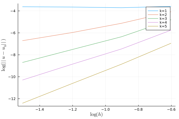
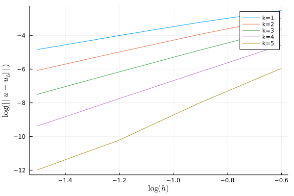
I assume the exact solution \(u(x,y) = x^2(1-x)^2y^2(1-y)^2\) and derive the function \(f(x,y)\) accordingly. For this choice, fortunately \(u = \nabla u\cdot \mathbf{n} = 0\) on the boundary. Here I show the results up until fifth order DG approximation. The codes are given below:
| \(i=3\) | \(i=1\) |
|---|---|
 |
 |
| Polynomial order | Rate | Polynomial order | Rate | |||
| 1 | [0.3852, -0.1930 -0.0916] | 1 | [2.3182, 2.6385, 2.7471] | |||
| 2 | [3.4888, 2.8130, 2.4539] | 2 | [3.1978, 3.5151, 3.5987] | |||
| 3 | [5.1583, 3.8862, 3.9024] | 3 | [4.1920, 4.3205, 4.3889] | |||
| 4 | [5.6954, 4.6425, 4.7674] | 4 | [5.2752, 5.3111, 5.3818] | |||
| 5 | [6.3395, 5.8784, 5.9436] | 5 | [6.7739, 7.4219, 5.8162] |
In the left-hand side, I show the results of the scheme discussed by Gudi et al. for \(i=3\). In the right-hand side, I show the results of the scheme with the modified penalty parameter \(i=1\). In the figures \(k\) denotes the polynomial order of approximation.
-
One thing that stands out immediately is the rate of convergence for piece-wise linear approximation. While setting \(i=3\) does not yield convergence for linear elements, \(i=1\) yields optimal (super?) convergence here.
-
For \(i=3\) we observe sub-optimal convergence in the \(L^2\) norm for piece-wise quadratic elements, while \(i=1\) yields optimal convergence. Although the magnitude of the error seems to be higher in \(i=1\) case. Interesting.
-
Higher order elements seem to yield optimal estimates (atleast close to) in both cases here. This is probably expected, as seen from the original article by Gudi et al..
So far the results are consistent with the observations of Gudi et al. for \(i=3\). There is something interesting happening when \(i=1\) in the penalty term.
Example 2
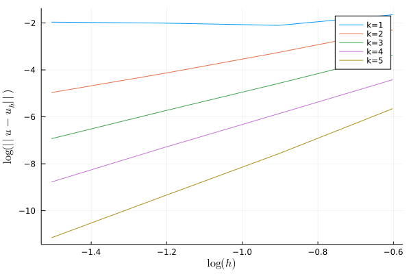
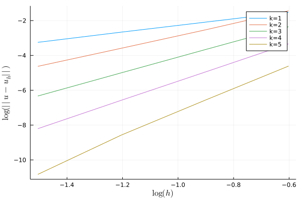
Let us run the tests for one more example, \(u(x,y) = sin(\pi x)\sin(\pi y)\). It is one of my favourite examples to test for convergence in elliptic FEM problems.
| \(i=3\) | \(i=1\) |
|---|---|
 |
 |
| Polynomial order | Rate | Polynomial order | Rate | |||
| 1 | [1.4976, -0.3135, -0.1474] | 1 | [1.9061, 1.8918, 1.9492] | |||
| 2 | [3.1732, 2.9442, 2.7414] | 2 | [3.6448, 3.4870, 3.4528] | |||
| 3 | [4.0097, 3.8762, 3.9568] | 3 | [4.3743, 4.4074, 4.4296] | |||
| 4 | [4.7994, 4.7530, 4.9161] | 4 | [5.3946, 5.3610, 5.4243] | |||
| 5 | [6.3664, 5.9323, 5.9673] | 5 | [6.5199, 6.6304, 7.5057] |
Mostly the same, except now for \(k=1\) i.e., linear polynomials we get the optimal rate of convergence when \(i=1\). It might be because the exact solution is not a polynomial. Again, the results seems consistent with Gudi et al. for \(k=3\).
Conclusions
In Symmetric Interior Penalty Galerkin (SIPG) Method, the choice of penalty parameter \(\sigma_0\) has mostly been an arbitrary real number that is sufficiently large. A definite lower bound to my knowledge has not yet been established. In this case for mixed DG method, however, an upper bound for the penalty term \(\alpha|_{e_k} = \sigma_0 |e_k|^{-i} p^2\) may exist. A high value (proportional to \(|e_k|^{-3}\)) may erode the method into producing sub-optimal rates. A low value (proportional to \(|e_k|^{-1}\)), and hence a low value of \(\sigma_0\) could explain the good rate of convergence.
While an improvement in the convergence is observed for linear elements when the penalty term is reduced (taken proportional to \(|e_k|^-1\)), the magnitude of the error for higher order elements seems to actually be higher when the penalty term is proportional to \(|e_k|^{-1}\) than when it is proportional to \(|e_k|^{-3}\). This also needs some more tests.
Update (14 Aug 2021)
I did some test for 3D problems and I observed similar results as in 2D. The exact solution I assumed is \(u(x,y,z) = x^4(1-x)^4y^4(1-y)^4z^4(1-z)^4\) on a unit cube.
| \(i=3\) | \(i=1\) | |||||
| Polynomial order | Rate | Polynomial order | Rate | |||
| 1 | [2.8811, 1.3726, -0.0986] | 1 | [2.0525, 2.2049, 2.4382] | |||
| 2 | [5.1508, 3.4932, 2.5361] | 2 | [3.8400, 3.6734, 4.7405] |
References
Gudi, T., Nataraj, N. & Pani, A.K. Mixed Discontinuous Galerkin Finite Element Method for the Biharmonic Equation. J Sci Comput 37, 139–161 (2008). https://doi.org/10.1007/s10915-008-9200-1
tags: wip - discontinuous - Galerkin - gridap © 2019- Balaje Kalyanaraman. Hosted on Github pages. Based on the Minimal Theme by orderedlist