
Postdoc at Umeå University, Sweden
Shape from Shading - Revisited
A few years ago, I worked on Hamilton Jacobi Equations at the Tata Institute of Fundamental Research as an undergraduate. One of the interesting applications of Hamilton Jacobi Equations is the shape from shading problem. I had a great time working with my mentor Prof. G.D.Veerappa Gowda and my friend Sanath Keshav on the project.
The problem demonstrates how powerful mathematics can be in modelling real-life scenario. With computers and new technologies now available, PDE-based models can be solved relatively easily which opens up a huge amount of possible applications. Recently, I got super interested in the theory of Hamilton Jacobi Equations including the well-posedness of the boundary value problem. In this post I would like to summarize briefly what I have learned and stuff I have worked on so far. I also intend to make a series of blog posts on this topic explaining the modelling and the mathematics that runs behind this problem.
What is Shape from Shading?
The problem is to compute the three-dimensional shape of a surface from one image of that surface. The image below shows the concept of shape from shading.
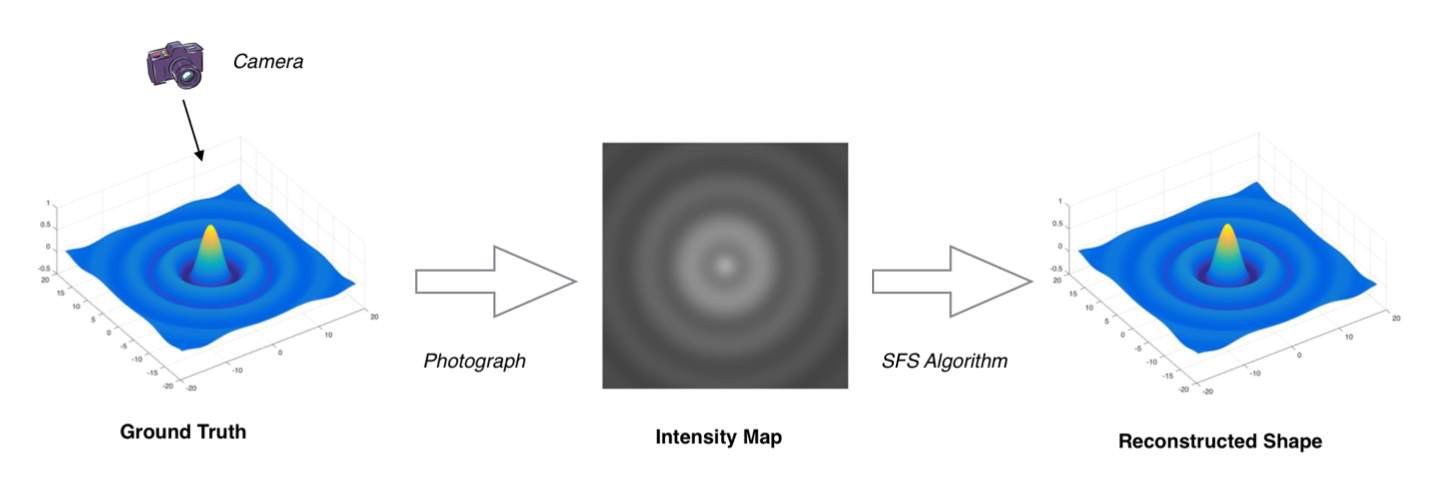 |
Several mathematical models have been proposed to study the shape from shading problem. All the models lead to a class of partial differential equations known as Hamilton Jacobi Equations. For more details about the construction of the model, I refer the reader to the article by E. Prados and O. Faugeras and the references therein.
All the models assume that the brightness value \(I(x,y)\) at each pixel is related to the reflectance of any surface \(R(n(x,y))\)
\[I(x,y) = R(n(x,y))\]The simplest one is the orthographic model which assumes that the object (Lambertian) is illuminated by a single distant light source. If \((0,0,-1)\) is the direction of illumination, then the reflectance is given by the equation
\[I(x,y) = R(n(x,y)) = \vec{L}\cdot\mathbf{n} = (0,0,-1)\cdot\mathbf{n} = (0,0,-1)\cdot\frac{(\frac{\partial u}{\partial x}, \frac{\partial u}{\partial y}, -1)}{\sqrt{1 + \left(\frac{\partial u}{\partial x}\right)^2 + \left(\frac{\partial u}{\partial y}\right)^2}}\]where \(\mathbf{n}\) is the unit normal vector of the reconstructed surface (our solution) \(u = u(x,y)\). Rearranging the equation and making \(u\) the subject of the equation, we obtain the PDE
\[|\nabla u| - \sqrt{\frac{1}{I(x,y)^2} - 1} = 0\]which is known as the Eikonal equation. The differential equation is usually combined with some boundary condition such as the Dirichlet boundary condition \(u = 0\).
Is it well-posed?
A common problem with the orthographic model is that the boundary value problem is ill-posed, i.e., there exists no unique solution. The problem is two folds here.
-
There exists no solution to the HJE in \(C^1\), meaning there is no differentiable solution. This can be proved using contradiction by a simple application of the Rolle’s theorem. The best space that we could look for solution is in \(C^0\). The problem is, there are infinite candidates for solutions in \(C^0\). Any function that is continuous whose absolute value of the derivative is equal to \(f(x)\) almost everywhere is a candidate. This can be remedied using the concept of viscosity solutions which places restrictions on the set of solutions we are looking for. Under this framework, we could narrow it down to two possible cases: a solution that is concave up and concave down. This brings us to the next problem:
-
The concave/convex ambiguity. At points where \(I=1\), the solution \(+u\) and \(-u\) can both be a solution to the problem. This leads to the concave/convex ambiguity which cannot be solved in the viscosity framework and hence leads to a loss of uniqueness.
This has been discussed in the paper by Elisabeth Rouy and Agnes Tourin
The (improved) perspective model
By assuming that the light source is not placed at infinity, but at some point away from the object, Prados and Faugeras came up with the model known as the perspective model. By taking the brightness equation
\[I(x,y) = \frac{\vec{L}\cdot\mathbf{n}}{r^2}\]where \(r\) is the distance between the light source and surface, Prados and Faugeras were able to show that the uniqueness issue can be circumvented. By adding the parameter \(r\) into the model, the convex/concave ambiguity is effectively removed, because a concave surface would have a higher value \(r\) than a convex surface \(r\). This leads to a HJE that is significantly more sophisticated
\[-e^{-2u} + \frac{I(\mathbf{x})f^2}{Q(\mathbf{x})}\sqrt{f^2|\nabla u|^2 + (\nabla u\cdot \mathbf{x})^2 + Q(\mathbf{x})^2} = 0\]where \(Q(x) = \sqrt{\frac{f^2}{f^2+\|\mathbf{x}\|^2}}\). This equation gives a powerful description of the shape from shading problem. And plus a provably convergent numerical scheme can be derived using the theory of Hamilton Jacobi Equations. The scheme is based on the one discuss by Rouy and Tourin in the paper
Let
\[H(x,u,\nabla u) = -e^{-2u} + \frac{I(\mathbf{x})f^2}{Q(\mathbf{x})}\sqrt{f^2|\nabla u|^2 + (\nabla u\cdot \mathbf{x})^2 + Q(\mathbf{x})^2}\]The pseudo-code of the Rouy and Tourin scheme is:
# Construct the Hamiltonian using the Rouy and Tourin Scheme

function H(i,j,U)
    :
    :

    # Construct the Gradient Approximation
    D₊ˣ = (U[i+1,j] - U[i,j])/Δx
    D₋ˣ = (U[i,j] - U[i-1,j])/Δx
    D₊ʸ = (U[i,j+1] - U[i,j])/Δy
    D₋ʸ = (U[i,j] - U[i,j-1])/Δy
    Dˣ = max(0, -D₊ˣ, D₋ˣ)
    Dʸ = max(0, -D₊ʸ, D₋ʸ)
    ∇u = [Dˣ, Dʸ]

    :
    :
end

ε = 1
tol = 1e-6

while ε > tol
    # Points in the interior
    for i=2:N-1
        for j=2:N-1


U₁[i,j] = U[i,j] - Δt*H(i,j,U)
        end
    end
end
Thats it! The Julia Language code is given below
The input image and the output of the code is given below
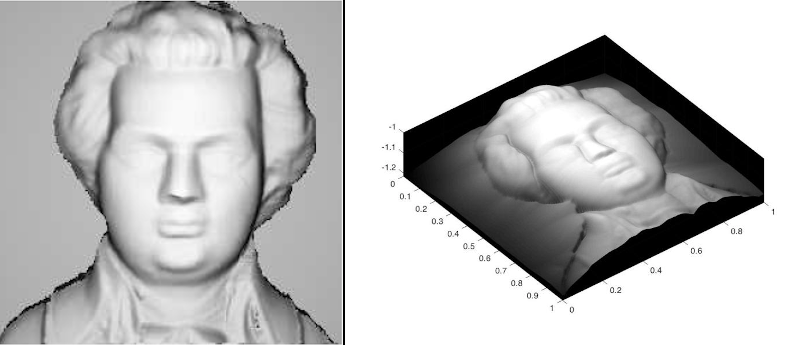 |
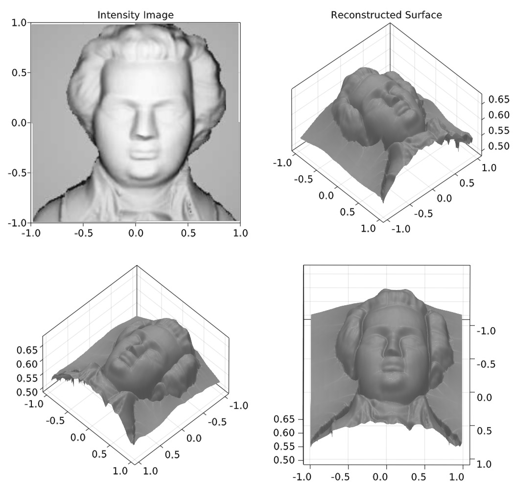 |
We also tried 3D printed the surface.
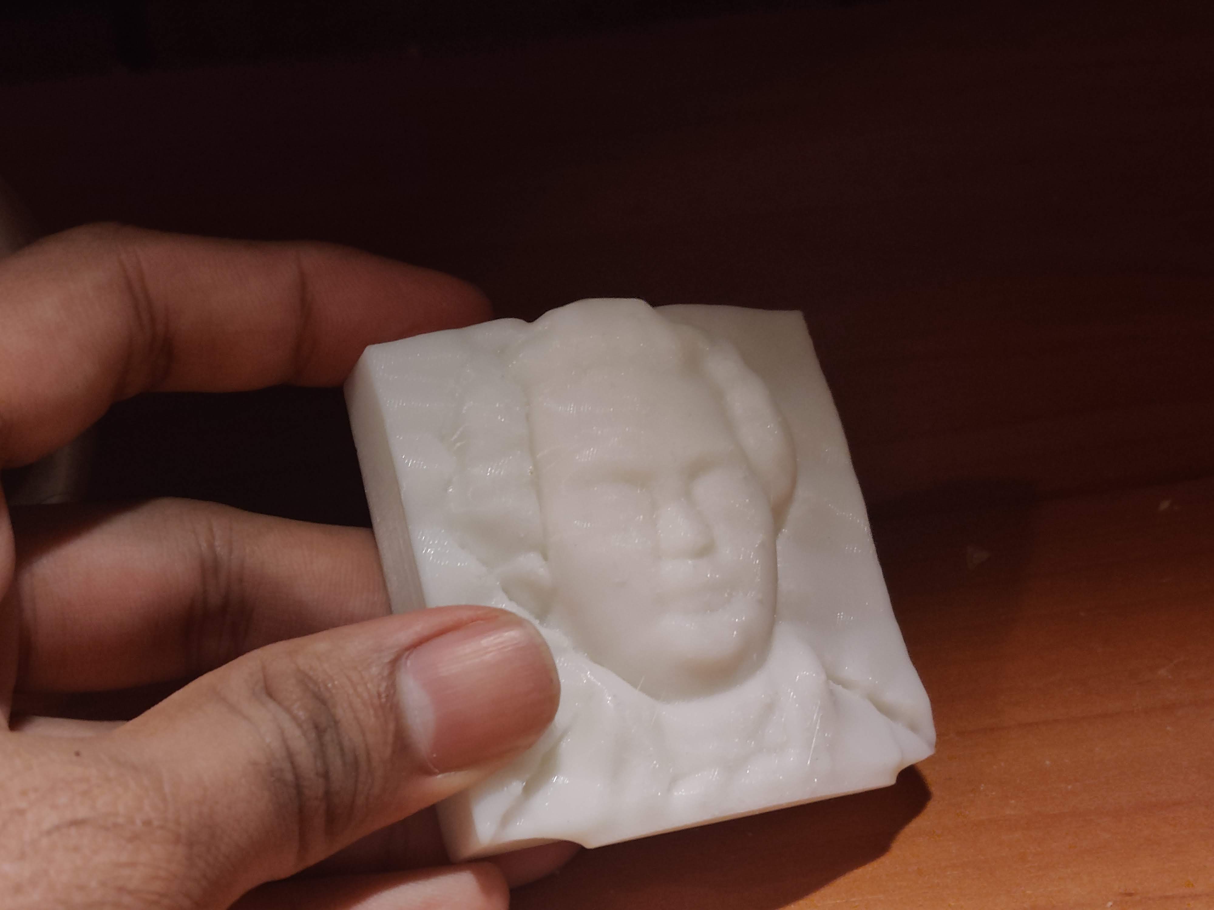 |