
Postdoc at Umeå University, Sweden
Ice Shelf Vibrations
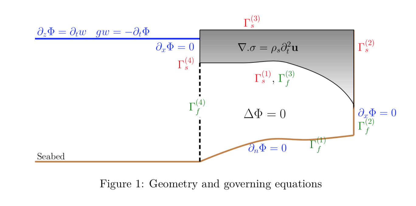 |
Consider an ice-shelf which is assumed to be a two dimensional elastic body. The ice-shelf is fixed at the landward end \(x=L\) (right) and free to vibrate at the seaward end \(x=0\) (left). Open ocean of depth \(H\) exists for \(x<0\) and a cavity region filled with water exists underneath the ice-shelf \(0<x<L\). The fluid flow is governed by the potential flow theory and the vibration of the ice-shelf is governed by linear-elasticity theory.
The objective of the problem is to study the vibrations of the ice-shelf in response to the waves generated in the open ocean region. The problem is solved using the finite element method and the displacement of the ice-shelf are shown in the videos below. The code is available on Github which was also published in the Journal of Open Source Software. The video below compares the vibration of an ice-shelf (modelled as a clamped elastic body) vs an iceberg (modelled as a free elastic body) subject to the same incident wave forcing. The semi-infinite boundary in Figure 1 is treated using a non-local boundary condition defined on the boundary \(\Gamma_f^{(4)}\). See the abstract of the presentation in 34th International Workshop on Water Waves and Floating Bodies and also my paper
Kalyanaraman, B., Meylan, M. H., Bennetts, L. G., & Lamichhane, B. P. (2020). A coupled fluid-elasticity model for the wave forcing of an ice-shelf. Journal of Fluids and Structures, 97, 103074.
Gradient Recovery for Virtual Element Methods
Gradient recovery methods are popular numerical techniques to approximate the gradient of the solution. They have super convergence property and are used in adaptive refinement. Gradient recovery techniques based on oblique projection are well studied for the finite element methods.
A gradient recovery technique based on the oblique projection can be defined for virtual element methods on Polygonal meshes. In the virtual element setting, the gradient recovery operator projects \(\nabla u_h\) by finding \(g_h^k = \text{Q}_h\left(\frac{\partial u_h}{\partial x_k}\right) \in V_h\) for \(k=1,2\) such that
\[\begin{equation} \sum_{K}\left(\Pi_K^{0}g_h^k, \Pi_K^{0} \mu_j\right)_K = \sum_{K}\left(\frac{\partial (\Pi_K^{0} u_h)}{\partial x_k}, \Pi_K^{0}\mu_j\right)_K. \end{equation}\]with \((x_1,x_2) = (x,y)\) and the functions \(\mu_j \in \mathcal{M}_h := \text{span}\{\mu_1,\mu_2,\cdots,\mu_N\}\) satisfy the bi-orthogonal relation
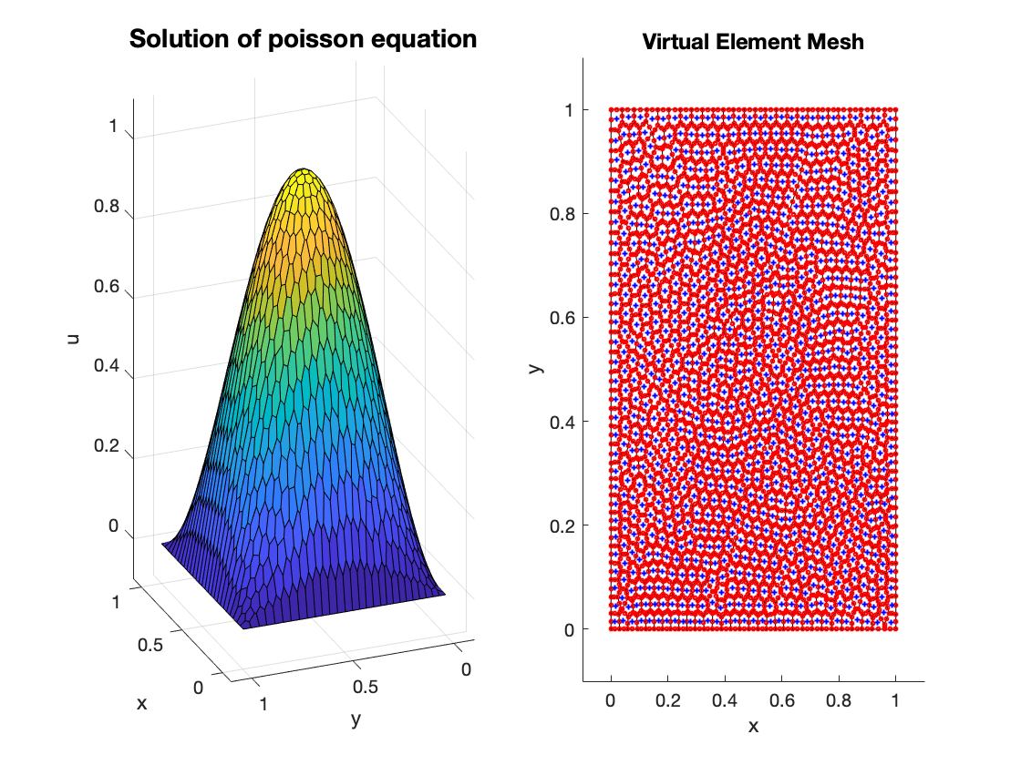
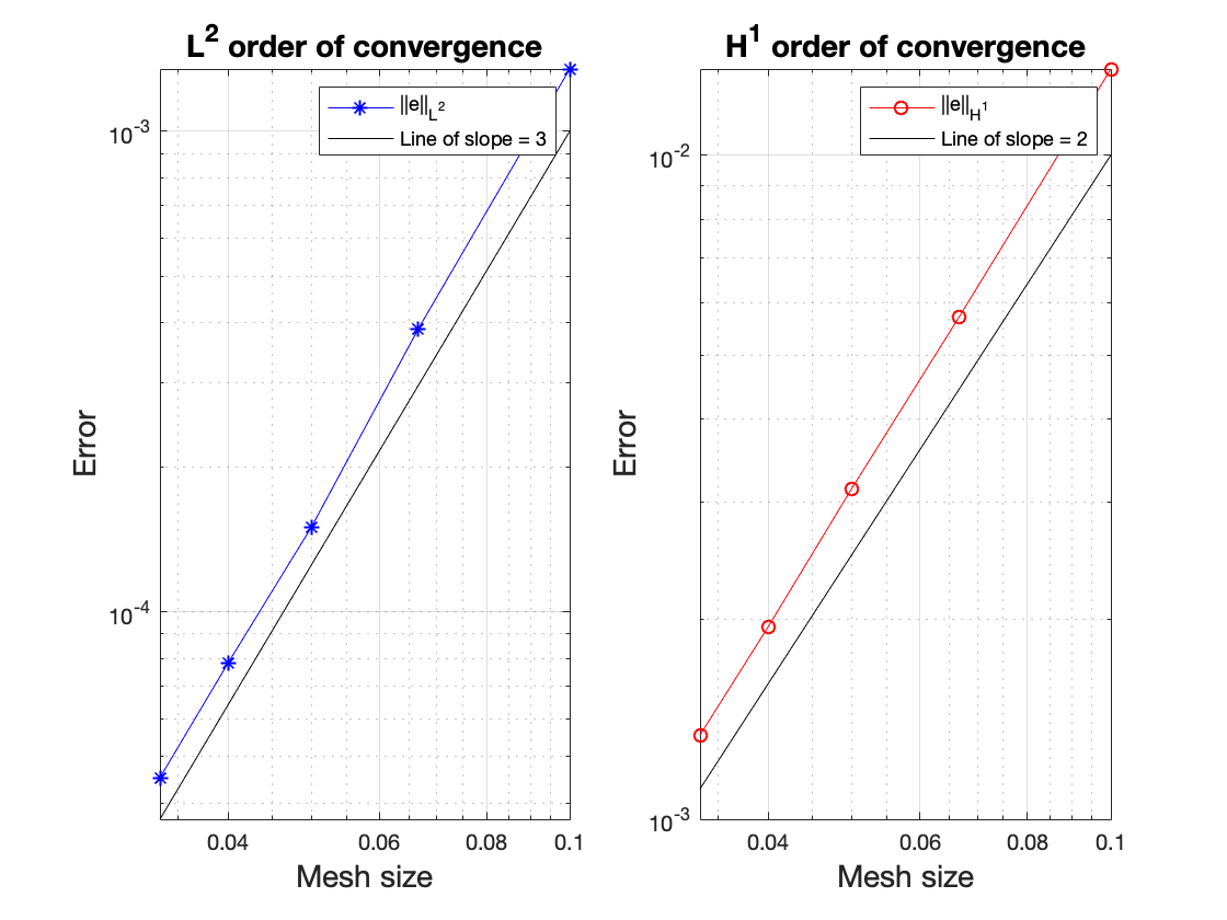
\[\begin{equation} \left(\Pi^{0}_K \varphi_i, \Pi^{0}_K \mu_j\right)_K = c_j \delta_{ij} \quad \forall K \in \mathcal{T}_h.\label{eq:biorth} \end{equation}\]where the scaling factors \(c_j\) are obtained using mass lumping. We can observe higher rates of convergence for the gradient which is shown in the Figure below.
 |
 |
You can find the full article online published in the ANZIAM Journal. Do read my blog post on how it can be made better!! Also, check out this repository for the MATLAB codes.
© 2019- Balaje Kalyanaraman. Hosted on Github pages. Based on the Minimal Theme by orderedlist