
Postdoc at Umeå University, Sweden
Generating Pretty Unicode Plots
A couple of months ago while I was learning Julia programming, I came across this tweet
Okay, this is one of the coolest #JuliaLang packages I've come across in a while. 💯 super nerd points go to UnicodePlots.jl for neat plotting directly in the terminal pic.twitter.com/aokc4CZpGb
— Milan Klöwer (@milankloewer) April 14, 2021
I don’t normally spend a lot of time on twitter, but when I saw this
tweet, I knew I needed to act upon this. I instantly fell in love with
this and I wanted to do something cool with it. I got the
Google Summer of Code with Gridap and started working on my
project. During the weekends when I wasn’t working on my GSoC project,
I continued to explore Gridap and Julia, and so a couple of
weeks ago, I decided to work on something with UnicodePlots.jl. I will
briefly talk about the mathematics that runs behind the code in the
following section. Feel free to skip to the next session if you want
to look at the implementation aspect.
Mathematical Model
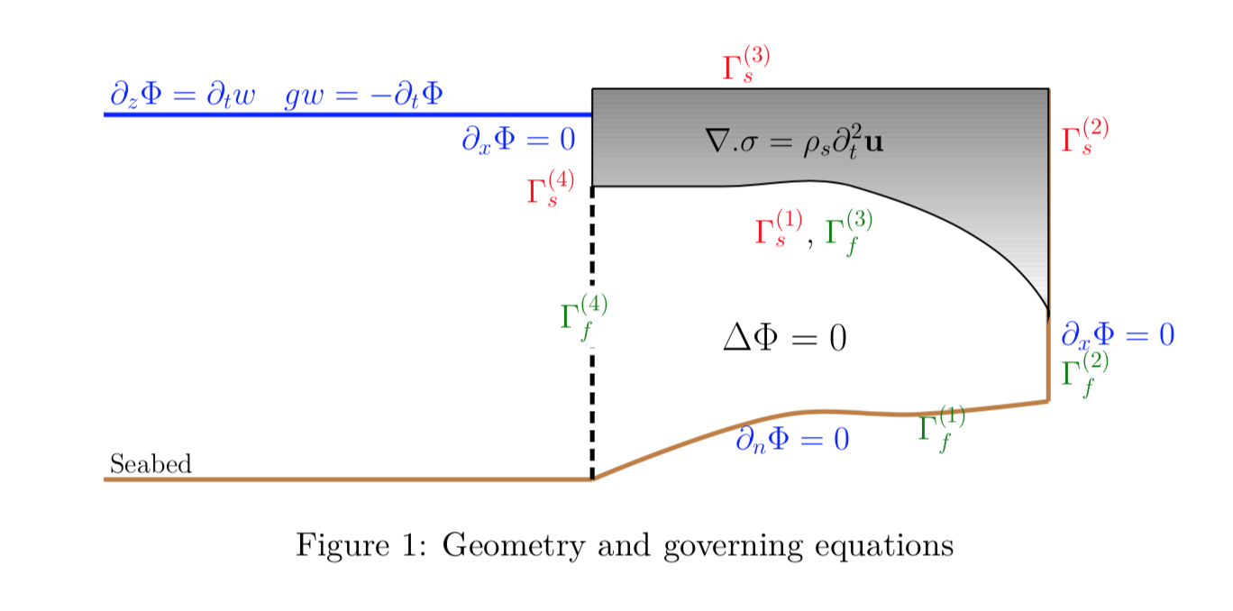 |
Consider the geometry and the schematic shown in the figure above. The motion of the ice-shelf (solid) is governed by the elastodynamic equations/thin-plate equation which are coupled with the fluid motion, governed using the linear potential flow theory. The fluid is modelled as a semi-infinite rectangular region of uniform depth, whereas the sub-shelf cavity region is assumed to be non-uniform. The time-domain problem is converted to the frequency domain by applying a transformation
\begin{equation} \Phi(x,z,t) = \mbox{Re} \left( \phi(x,z)e^{-i \omega t} \right),\quad \mathbf{u}(x,z,t) = \mbox{Re}\left( \eta(x,z)e^{-i \omega t} \right) \end{equation}
at a prescribed frequency \(\omega\). The semi-infinite region is truncated by constructing analytic expressions of the form
\begin{equation} \phi(x,z) = \tau_{0}(x,z) \, e^{-i k_0x} + c_0 \;\tau_0(x,z)\,e^{i k_0 x} + \sum_{m=1}^{M} c_m \;\tau_m(x,z)\,e^{i k_m x} \end{equation}
The constants \(k_m\) are the wave numbers, and \(k_0\) is the leading wave-number, all satisfying the well known dispersion equation.
\begin{equation} -k\, \tan\,kH = \frac{\omega^2}{g} \end{equation}
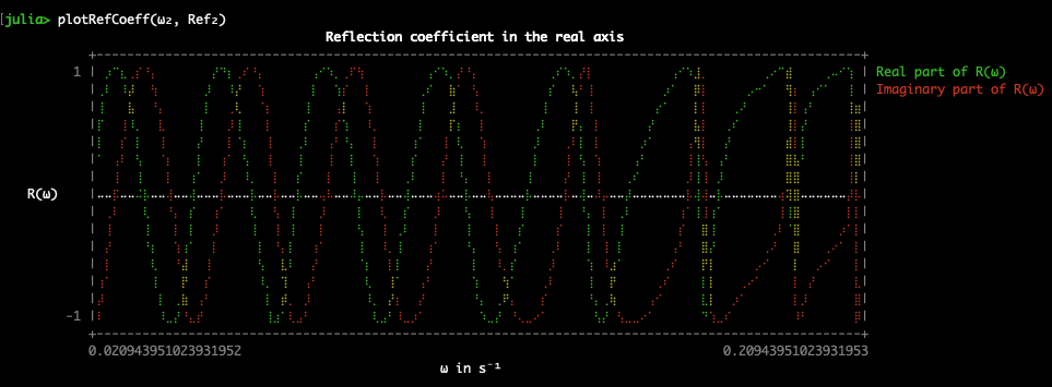
The number \(c_0\) is the reflection coefficient, which is actually the amplitude of the reflected wave. I set my end goal to generate this picture (or atleast something close to it).
 |
This is the plot of the reflection coefficient \(c_0\) in the complex plane as a function of incident frequency \(\omega\). The reflection coefficient is the amplitude of the reflected wave. You can check out my paper if you wish to know more.
Ilyas, M., Meylan, M. H., Lamichhane, B., & Bennetts, L. G. (2018). Time-domain and modal response of ice shelves to wave forcing using the finite element method. Journal of Fluids and Structures, 80, 113–131.
The first step is to solve the governing equations using the finite element method. The goal is to compute the matrix
\begin{equation} H(\omega) = [\mathbf{K}-\omega^2\mathbf{M}+i\omega\mathbf{B}]{\lambda} = {\mathbf{f}} \end{equation} where the entries of the matrices are given by
\[\begin{eqnarray} \mathbf{K}_{jk} = \left(\sigma(\eta_j)\,:\,\epsilon(\eta_k)\right)_{\Omega_s},&\quad \mathbf{M}_{jk} = \rho_s(\eta_j,\eta_k)_{\Omega_s}, \\ \mathbf{C}_{jk} = \left\langle\eta_j,\eta_k\cdot\mathbf{n}\right\rangle_{\Gamma_s^{(1)}},&\quad \mathbf{B}_{jk} = \left\langle\phi_j,\eta_k\right\rangle_{\Gamma_f^{(3)}}. \end{eqnarray}\]-
The potential \(\phi_0\) is the motion of the fluid when the ice-shelf acts as a rigid body without motion. The quantities \(\eta_j\) are the in-vacuo vibration modes of the ice-shelf. The motion of the ice-shelf are independent of frequency \(\omega\). This can be obtained by the finite element method. If using the thin-plate theory, the modes of the ice can be obtained by analytic expressions for cantilever modes.
-
Corresponding to \(\eta_j\), the motion of the fluid is described by the radiation potentials \(\phi_j\). All these quantities can be obtained using the finite element method for arbitrary fluid geometries.
The crucial property is that these quantities are analytic functions of the incident frequency \(\omega\). Thus the entries of the matrix \(H(\omega)\) are analytic functions. Once few entries are obtained in the frequency space, using this property, we can interpolate the entries over a finer frequency space. All the numerics were handled mostly using Gridap. There’s more …
Gridap.jl and UnicodePlots.jl
The full code is available in this repository here. The necessary dependencies are listed below:
Gridap # For Finite Element Method
Arpack # Optional. Since I use Euler-Bernoulli currently
Roots # To solve the dispersion equations
SparseArrays # For storing external sparse matrices
Interpolations # For interpolation
UnicodePlots # Terminal related plotting
ComplexPhasePortrait # Domain coloring for complex functions
To load the necessary functions in the REPL, we run
julia> include("ice.jl");
An example problem is provided in the script example.jl.
julia> include("example.jl");
Once the reflection coefficients in the frequency space are obtained,
plotting is mostly straightforward. I have included some plotting
routines to make this a little easier for first time users. Then
simply run (if using example.jl)
julia> plotRefCoeff(ω₂, Ref₂)
julia> plotComplexRefCoeff(a,b,c,d,Ref₃)
And you get these:
 |
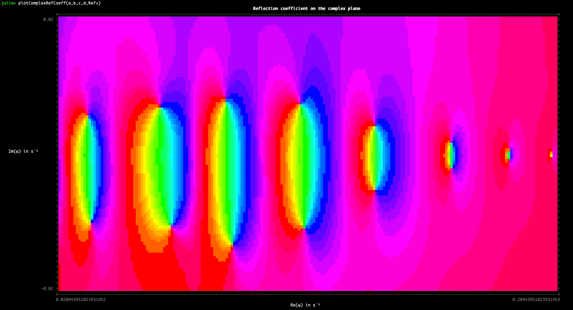 |
Impressive! (I made the font size small for the complex plot to get more detail in the terminal).
Multiple Dispatch
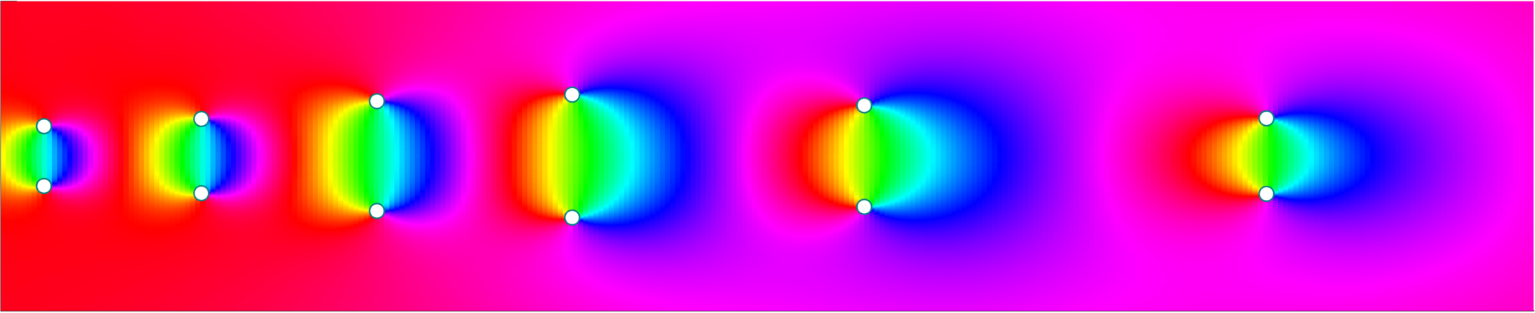
I want to spend a section here to talk about the one of the best features of Julia Language and how it works. Multiple dispatch.
In this code snippet,
using UnicodePlots
using ComplexPhasePortrait

nx = 1000
x = range(-1, stop=1, length=nx)
Z = x' .+ reverse(x)*im

f = z -> (z - 0.5im)^2 * (z + 0.5+0.5im)/z
fz = f.(Z)

img = portrait(fz)
heatmap(img,width=80,height=80)
multiple dispatch occurs when I write
img = portrait(fz)
heatmap(img,width=80,height=80)
and I am able to generate the complex plot. In a nutshell …
The function
portrait()is a part of theComplexPhasePortraitpackage andheatmap()is part of theUnicodePlotspackage. The functionportrait()returns anRGBtriplet of the associated phase plot. Passing the output of this function toheatmap()directly plots this without any issues. This is because the input argument ofheatmap()is in fact a subtype of the output produced byportrait(). This is particularly impressive as the developers of the two packages are totally different groups. Meaning that the developers ofComplexPhasePortraitneed not contact the developers ofUnicodePlotsto make sure that the data-types are consistent between the functions.
I even tweeted this and people seem to like it!
Complex Phase Portraits using UnicodePlots.jl! Reflection coefficients (amplitude of the reflected wave) as a function of frequency in the real vs. complex space.
— Balaje K (@BalajeKkb) July 2, 2021
Built using #gridap #julialang @JuliaLanguage and many more! Code 👇https://t.co/YZyFdNONbz#FEM #opensource pic.twitter.com/myWJoT6ey7
My next side project would be to generate some movies in the terminal
using the VideoInTerminal.jl
package. I
think I may generate the time-domain simulations for the ice-shelf
motion. That should be fun!
So yeah. That’s it for this blog post, I will catch you guys in the next one.
tags: iceshelf - unicodeplots © 2019- Balaje Kalyanaraman. Hosted on Github pages. Based on the Minimal Theme by orderedlist